GObayesC Report
Last updated: 2023-12-05
Checks: 7 0
Knit directory: dgrp-starve/
This reproducible R Markdown analysis was created with workflowr (version 1.7.1). The Checks tab describes the reproducibility checks that were applied when the results were created. The Past versions tab lists the development history.
Great! Since the R Markdown file has been committed to the Git repository, you know the exact version of the code that produced these results.
Great job! The global environment was empty. Objects defined in the global environment can affect the analysis in your R Markdown file in unknown ways. For reproduciblity it’s best to always run the code in an empty environment.
The command set.seed(20221101) was run prior to running the code in the R Markdown file. Setting a seed ensures that any results that rely on randomness, e.g. subsampling or permutations, are reproducible.
Great job! Recording the operating system, R version, and package versions is critical for reproducibility.
Nice! There were no cached chunks for this analysis, so you can be confident that you successfully produced the results during this run.
Great job! Using relative paths to the files within your workflowr project makes it easier to run your code on other machines.
Great! You are using Git for version control. Tracking code development and connecting the code version to the results is critical for reproducibility.
The results in this page were generated with repository version f12f92f. See the Past versions tab to see a history of the changes made to the R Markdown and HTML files.
Note that you need to be careful to ensure that all relevant files for the analysis have been committed to Git prior to generating the results (you can use wflow_publish or wflow_git_commit). workflowr only checks the R Markdown file, but you know if there are other scripts or data files that it depends on. Below is the status of the Git repository when the results were generated:
Ignored files:
    Ignored:    .snakemake/
    Ignored:    code/methodComp/bglr/err-bglr-f.5381.err
    Ignored:    code/methodComp/bglr/err-bglr-m.5382.err
    Ignored:    code/methodComp/m/meth-m.4676.err
    Ignored:    code/methodComp/m/meth-m.4685.err
    Ignored:    code/methodComp/method-f.4751.out
    Ignored:    data/fb/
    Ignored:    data/snake/
    Ignored:    snake/.snakemake/
    Ignored:    snake/GOfile.yaml
    Ignored:    snake/ReadMe.md
    Ignored:    snake/Snakefile.yaml
    Ignored:    snake/bayesCheck.R
    Ignored:    snake/bayesTest.Rds
    Ignored:    snake/binner2.R
    Ignored:    snake/code/misc/
    Ignored:    snake/data/
    Ignored:    snake/datafile.yaml
    Ignored:    snake/dgrp.yaml
    Ignored:    snake/f_file.yaml
    Ignored:    snake/goNames.sh
    Ignored:    snake/goPost/
    Ignored:    snake/gofig.yaml
    Ignored:    snake/gospace.R
    Ignored:    snake/h2_synth.R
    Ignored:    snake/labMake.R
    Ignored:    snake/logs/
    Ignored:    snake/meta.sh
    Ignored:    snake/metaList
    Ignored:    snake/newlines
    Ignored:    snake/note1
    Ignored:    snake/pipelines/
    Ignored:    snake/rawHits
    Ignored:    snake/s1.sh
    Ignored:    snake/s2.sh
    Ignored:    snake/s3.sh
    Ignored:    snake/slurm/
    Ignored:    snake/smake.sbatch
    Ignored:    snake/snubnose.sbatch
    Ignored:    snake/srfile.yaml
    Ignored:    snake/temp9/
    Ignored:    snake/temporaire-rewrite.R
    Ignored:    snake/trimHits
    Ignored:    snake/vavrfile.yaml
    Ignored:    snake/vavrmake
    Ignored:    snake/zz_lost/
    Ignored:    zz_lost/

Untracked files:
    Untracked:  analysis/allotter.R
    Untracked:  analysis/old_index.Rmd.Rmd
    Untracked:  forester.R
    Untracked:  malegofind.R
    Untracked:  pippinRMDbackup.R
    Untracked:  snake/code/binner.R
    Untracked:  snake/code/combine_GO.R
    Untracked:  snake/code/dataFinGO.R
    Untracked:  snake/code/datafile.yaml
    Untracked:  snake/code/filterNcombine_GO.R
    Untracked:  snake/code/filter_GO.R
    Untracked:  snake/code/go/
    Untracked:  snake/code/method/bayesHome.R
    Untracked:  snake/code/method/multiplotGO.Rmd
    Untracked:  snake/code/method/sparse.R
    Untracked:  snake/code/srfile.yaml

Unstaged changes:
    Modified:   analysis/Method/BayesC.Rmd
    Modified:   analysis/bigGO.Rmd
    Modified:   snake/code/method/bayesGO.R
    Modified:   snake/code/method/goFish.R
    Modified:   snake/code/method/varbvs.R
Note that any generated files, e.g. HTML, png, CSS, etc., are not included in this status report because it is ok for generated content to have uncommitted changes.
These are the previous versions of the repository in which changes were made to the R Markdown (analysis/goReport.Rmd) and HTML (docs/goReport.html) files. If you’ve configured a remote Git repository (see ?wflow_git_remote), click on the hyperlinks in the table below to view the files as they were in that past version.
| File | Version | Author | Date | Message |
|---|---|---|---|---|
| Rmd | f12f92f | nklimko | 2023-12-05 | wflow_publish(“analysis/goReport.Rmd”) |
| html | 9d7a980 | nklimko | 2023-11-29 | Build site. |
| Rmd | 624825a | nklimko | 2023-11-29 | wflow_publish(“analysis/goReport.Rmd”) |
| html | 5585964 | nklimko | 2023-11-28 | Build site. |
| Rmd | c608e9c | nklimko | 2023-11-28 | wflow_publish(“analysis/goReport.Rmd”) |
| html | f43d423 | nklimko | 2023-11-28 | Build site. |
| Rmd | d2b97de | nklimko | 2023-11-28 | wflow_publish(“analysis/goReport.Rmd”) |
| html | 2230527 | nklimko | 2023-11-28 | Build site. |
| Rmd | 979c389 | nklimko | 2023-11-28 | wflow_publish(“analysis/goReport.Rmd”) |
| html | fa620e8 | nklimko | 2023-11-28 | Build site. |
| Rmd | 7c77c72 | nklimko | 2023-11-28 | wflow_publish(“analysis/goReport.Rmd”) |
| html | fe88a0c | nklimko | 2023-11-28 | Build site. |
| Rmd | 3dd7953 | nklimko | 2023-11-28 | wflow_publish(“analysis/goReport.Rmd”) |
| html | 12d6df4 | nklimko | 2023-11-28 | Build site. |
| Rmd | feaa8df | nklimko | 2023-11-28 | wflow_publish(“analysis/goReport.Rmd”) |
| html | 8ab4763 | nklimko | 2023-11-28 | Build site. |
| Rmd | 2e7171f | nklimko | 2023-11-28 | wflow_publish(“analysis/goReport.Rmd”) |
#setwd("..")

#Correlation Coefficient Paths
uniF <- readRDS('snake/data/go/40_all/sexf/partData.Rds')
uniM <- readRDS('snake/data/go/40_all/sexm/partData.Rds')
#reorders 50 X m table to a (50*m) X 2 table
#converts method into factor to retain order
ggTidy <- function(data){
for(i in 1:dim(data)[2]){
name <- colnames(data)[i]
temp <- cbind(rep(name, dim(data)[1]), data[,i, with=FALSE])
if(i==1){
hold <- temp
} else{
hold <- rbind(hold, temp, use.names=FALSE)
}
}
colnames(hold) <- c("method", "cor")
hold$method <- factor(hold$method, levels=unique(hold$method))
return(hold)
}
#wrapper for ggplot call to custom fill sex, title, and y axis label
ggMake <- function(data, sex, custom.title, custom.Ylab){
plothole <- ggplot(data, aes(x=method, y=cor, fill=method)) +
geom_violin(color = NA, width = 0.65) +
geom_boxplot(color='#440154FF', width = 0.15) +
theme_minimal() +
stat_summary(fun=mean, color='#440154FF', geom='point',
shape=18, size=3, show.legend=FALSE) +
labs(x=NULL,y=custom.Ylab, tag=sex, title=custom.title) +
theme(legend.position='none',
axis.text.x = element_text(angle = -45, size=10),
text=element_text(size=10),
plot.tag = element_text(size=15)) +
scale_fill_viridis(begin = 0.4, end=0.9,discrete=TRUE)
return(plothole)
}
corSummary <- function(dataList, outPath){
hold <- readRDS(dataList[1])
for (i in 2:length(dataList)) {
#print(i)
hold <- rbind(hold, readRDS(dataList[i]))
}
colnames(hold) <- c('sex', 'rmax', 'rgo', 'term', 'cor')
saveRDS(hold, outPath)
}partMake <- function(data, sex, yint1, cutoff, lower, custom.title, custom.Xlab, custom.Ylab){
plothole <- ggplot(data,aes(y=cor,x=term))+
geom_point(color=viridis(1, begin=0.5))+
geom_text(aes(label=ifelse(cor>cutoff, as.character(term),'')), hjust=-0.1, size=2, angle=90)+
geom_text(aes(label=ifelse(cor<lower, as.character(term),'')), hjust=-0.1, size=2, angle=90)+
geom_hline(yintercept = yint1) +
geom_hline(yintercept = cutoff) +
theme_minimal() +
labs(x=custom.Xlab,y=custom.Ylab, tag=sex, title=custom.title) +
theme(text=element_text(size=10),
plot.tag = element_text(size=15))
return(plothole)
}
dMake <- function(data, sex, custom.title, custom.Xlab, custom.Ylab, psize){
plothole <- ggplot(data, aes(x= index, y=cor, label=gene))+
geom_point(color=viridis(1, begin=0.5), size=psize)+
geom_text(aes(label=ifelse(cor>0.5, as.character(gene),'')),hjust=1,vjust=0, angle=90, size=3)+
theme_minimal() +
labs(x=custom.Xlab,y=custom.Ylab, tag=sex, title=custom.title) +
theme(text=element_text(size=8),
plot.tag = element_text(size=15))
return(plothole)
}Initial results showed that Gene Ontology association could be used to improve prediction accuracy of a Bayesian model by assigning genes of interest a separate portion of variance. The following results are from selecting GO terms with five or more associated genes and scoring their prediction accuracy as a mean of 25 replicates apiece.
allNames <- read.table(file="snake/goPost/dataList", sep="")
dataList <- allNames[,1]

front <- 'snake/data/go/33_metric/sexf/rmax0.8/rgo0.01/'
end <- '/rowData.Rds'

finalList <- paste0(front, dataList, end)

outPath <- 'snake/data/go/40_all/sexf/partData.Rds'

temp <- na.omit(readRDS(outPath))

facs <- matrix(as.factor(unlist(temp[,1:4])), ncol=4)
cors <- as.numeric(unlist(temp[,5]))

data <- data.table(facs, cors)
colnames(data) <- c('sex', 'rmax', 'rgo', 'term', 'cor')

dataF <- data[data$sex=='f',]

yintData1 <- readRDS('snake/data/sr/33_metric/go/sexf/rmax0.8/rgo0/term1/rowData.Rds')
yF <- as.numeric(yintData1[5])

#
gg[[1]] <- partMake(dataF, 'F', yF, 0.36, 0.27, 'Effect of GO Annotations in Bayesian models', 'GO Term', 'Prediction Accuracy')

dataFOF <- dataF[order(cor),]
#post processing
temp99 <- readRDS("snake/data/go/40_all/sexf/partData.Rds")

subF <- dataF[cor>0.36,4:5]

subF <- subF[order(-cor),]
#
#plot(x=1:dim(dataFOF)[1], y=dataFOF$cor)
#snake/
allNames <- read.table(file="snake/goPost/dataList", sep="")
dataList <- allNames[,1]
front <- 'snake/data/go/33_metric/sexm/rmax0.8/rgo0.01/'
end <- '/rowData.Rds'
finalList <- paste0(front, dataList, end)
outPath <- 'snake/data/go/40_all/sexm/partData.Rds'
temp <- na.omit(readRDS(outPath))
facs <- matrix(as.factor(unlist(temp[,1:4])), ncol=4)
cors <- as.numeric(unlist(temp[,5]))
data <- data.table(facs, cors)
colnames(data) <- c('sex', 'rmax', 'rgo', 'term', 'cor')
dataM <- data[data$sex=='m',]
yintData1 <- readRDS('snake/data/sr/33_metric/go/sexm/rmax0.8/rgo0/term1/rowData.Rds')
yM <- as.numeric(yintData1[5])
#
gg[[2]] <- partMake(dataM, 'M', yM, 0.48, 0.40, 'Effect of GO Annotations in Bayesian models', 'GO Term', 'Prediction Accuracy')
dataMOM <- dataM[order(cor),]
#post processing
#temp99 <- readRDS("snake/data/go/40_all/sexm/partData.Rds")
subM <- dataM[cor>0.48,4:5]
subM <- subM[order(-cor),]
#plot(x=1:dim(dataFOF)[1], y=dataFOF$cor)termReader <- function(term, sex)
{
idPath <- paste0('snake/data/go/03_goterms/sex', sex,'/', term, '.Rds')
fitPath <- paste0('snake/data/go/25_fit/sex', sex,'/', term, '/bayesFull.Rds')
xpPath <- paste0('snake/data/01_matched/', sex,'_starvation.Rds')
xp <- readRDS(xpPath)
genes <- colnames(xp[,-1])
id1 <- readRDS(idPath)
model1 <- readRDS(fitPath)
fit1 <- model1$fit
inlay <- fit1$ETA[[1]]$d
outlay <- fit1$ETA[[2]]$d
fitDataM <- data.table(index=c(1:length(inlay)), cor=inlay, gene=genes[id1])
plothole <- dMake(fitDataM, toupper(sex), paste0(term, " PIP"), 'Index', 'PIP', 1)
return(plothole)
}
f1 <- termReader('GO.0045819', 'f')
f2 <- termReader('GO.0033500', 'f')
f3 <- termReader('GO.0055088', 'f')
f4 <- termReader('GO.0042675', 'f')
m1 <- termReader('GO.0035008', 'm')
m2 <- termReader('GO.0140042', 'm')
m3 <- termReader('GO.0007485', 'm')
m4 <- termReader('GO.0005811', 'm')nonReader <- function(term, sex){
idPath <- paste0('snake/data/go/03_goterms/sex', sex,'/', term, '.Rds')
fitPath <- paste0('snake/data/go/25_fit/sex', sex,'/', term, '/bayesFull.Rds')
xpPath <- paste0('snake/data/01_matched/', sex,'_starvation.Rds')
xp <- readRDS(xpPath)
genes <- colnames(xp[,-1])
id1 <- readRDS(idPath)
model1 <- readRDS(fitPath)
fit1 <- model1$fit
inlay <- fit1$ETA[[1]]$d
outlay <- fit1$ETA[[2]]$d
fitDataM <- data.table(index=c(1:length(outlay)), cor=outlay, gene=genes[-id1])
plothole <- dMake(fitDataM, toupper(sex), paste0(term, " PIP"), 'Index', 'PIP', 0.1)
return(plothole)
}
nf1 <- nonReader('GO.0045819', 'f')
nf2 <- nonReader('GO.0033500', 'f')
nf3 <- nonReader('GO.0055088', 'f')
nf4 <- nonReader('GO.0042675', 'f')
nm1 <- nonReader('GO.0035008', 'm')
nm2 <- nonReader('GO.0140042', 'm')
nm3 <- nonReader('GO.0007485', 'm')
nm4 <- nonReader('GO.0005811', 'm')Female
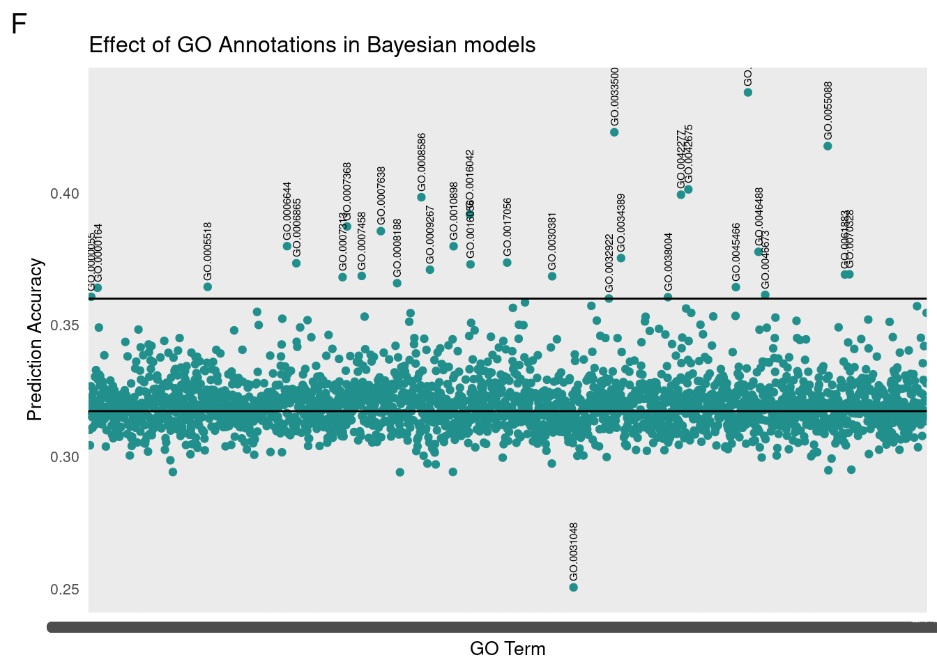
Top Results
print(subF) term cor
1: GO.0045819 0.4382497
2: GO.0033500 0.4231229
3: GO.0055088 0.4178735
4: GO.0042675 0.4014416
5: GO.0042277 0.3994211
6: GO.0008586 0.3984704
7: GO.0016042 0.3919625
8: GO.0007368 0.3873729
9: GO.0007638 0.3856025
10: GO.0006644 0.3799043
11: GO.0010898 0.3798619
12: GO.0046488 0.3777651
13: GO.0034389 0.3753829
14: GO.0017056 0.3736580
15: GO.0006865 0.3734180
16: GO.0016056 0.3729896
17: GO.0009267 0.3709695
18: GO.0070328 0.3692209
19: GO.0061883 0.3691317
20: GO.0007458 0.3686037
21: GO.0030381 0.3684766
22: GO.0007313 0.3681358
23: GO.0008188 0.3658592
24: GO.0005518 0.3644649
25: GO.0045466 0.3643595
26: GO.0000164 0.3641153
27: GO.0046673 0.3614228
28: GO.0000055 0.3606683
29: GO.0038004 0.3605215
30: GO.0032922 0.3600324
term corPosterior Inclusion Probability of GO portion
plot_grid(f1, f2, f3, f4, ncol=2)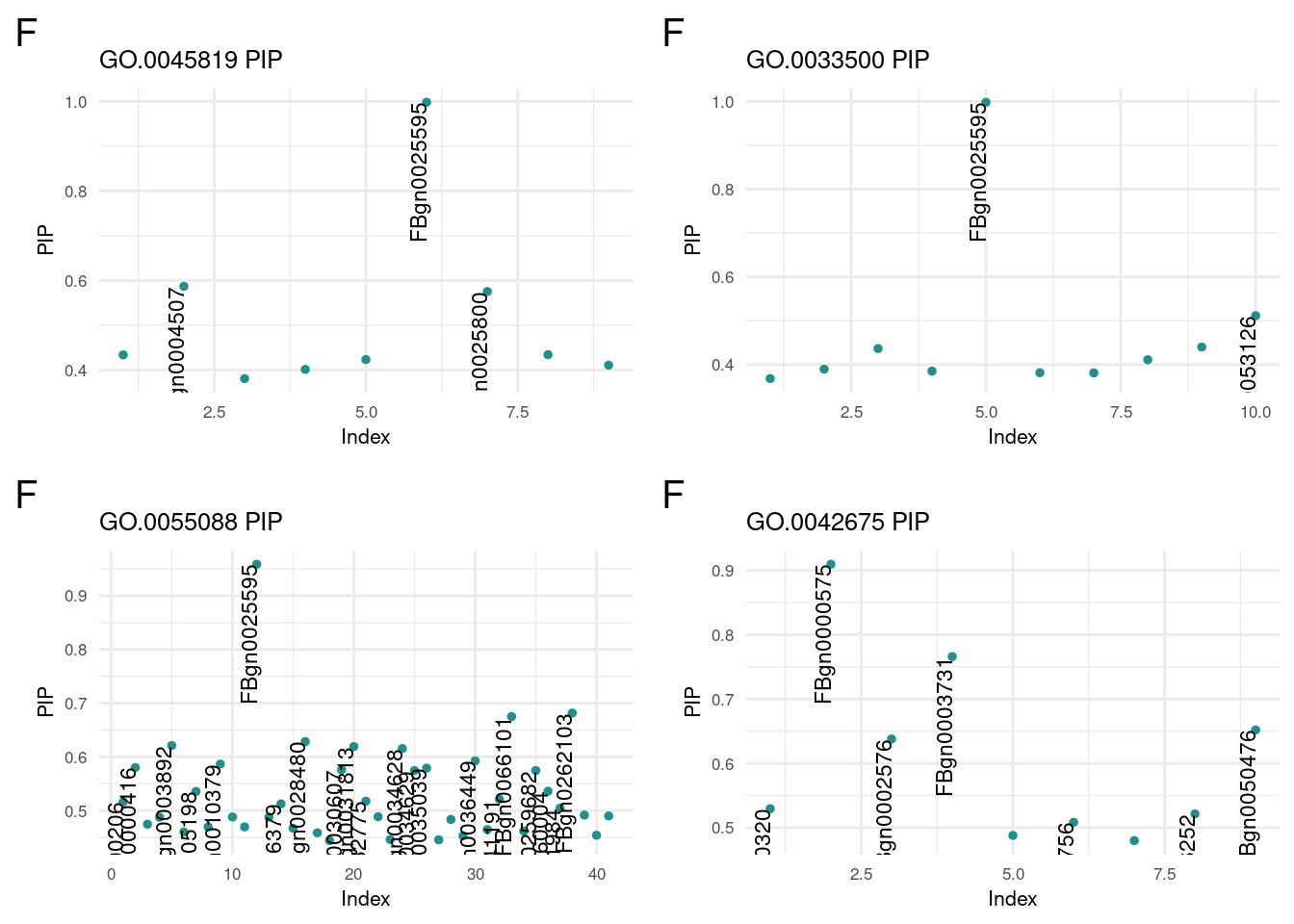
Posterior Inclusion Probability of non-GO portion
plot_grid(nf1, nf2, nf3, nf4, ncol=2)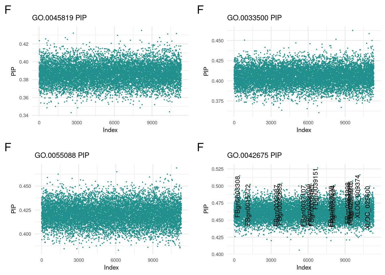
A detailed look at all PIP plots can be found here.
The low female outlier is GO:0031408 responsible for oxylipin synthesis.
We then translated the top GO terms into human readable categories to assess our findings. Below are the top ten ordered by correlation:
id: GO:0045819 name: positive regulation of glycogen catabolic process
id: GO:0033500 name: carbohydrate homeostasis
id: GO:0055088 name: lipid homeostasis
id: GO:0042675 name: compound eye cone cell differentiation
id: GO:0042277 name: peptide binding
id: GO:0008586 name: imaginal disc-derived wing vein morphogenesis
id: GO:0016042 name: lipid catabolic process
id: GO:0007368 name: determination of left/right symmetry
id: GO:0007638 name: mechanosensory behavior
id: GO:0006644 name: phospholipid metabolic process
Male
Overall
plot_grid(gg[[2]], ncol=1)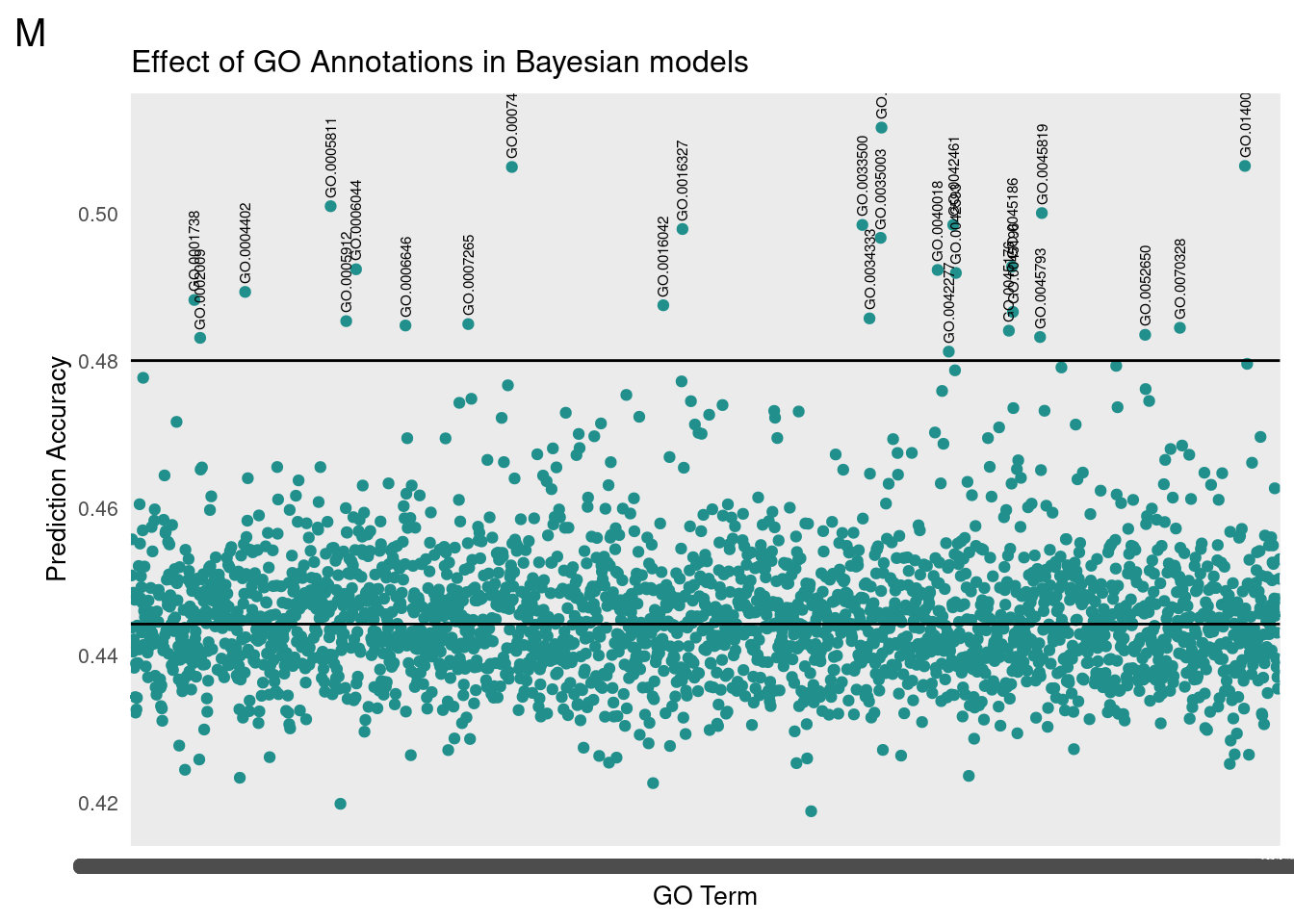
Top Results
print(subM) term cor
1: GO.0035008 0.5116379
2: GO.0140042 0.5064311
3: GO.0007485 0.5062906
4: GO.0005811 0.5009641
5: GO.0045819 0.5000330
6: GO.0042461 0.4984272
7: GO.0033500 0.4984207
8: GO.0016327 0.4978650
9: GO.0035003 0.4966652
10: GO.0045186 0.4927519
11: GO.0006044 0.4924000
12: GO.0040018 0.4923077
13: GO.0042593 0.4918994
14: GO.0004402 0.4893254
15: GO.0001738 0.4882313
16: GO.0016042 0.4875109
17: GO.0045196 0.4866070
18: GO.0034333 0.4857293
19: GO.0005912 0.4853594
20: GO.0007265 0.4849572
21: GO.0006646 0.4847660
22: GO.0070328 0.4844510
23: GO.0045176 0.4840628
24: GO.0052650 0.4835012
25: GO.0045793 0.4831989
26: GO.0002009 0.4830880
27: GO.0042277 0.4812196
term corPosterior Inclusion Probability of GO portion
plot_grid(m1, m2, m3, m4, ncol=2)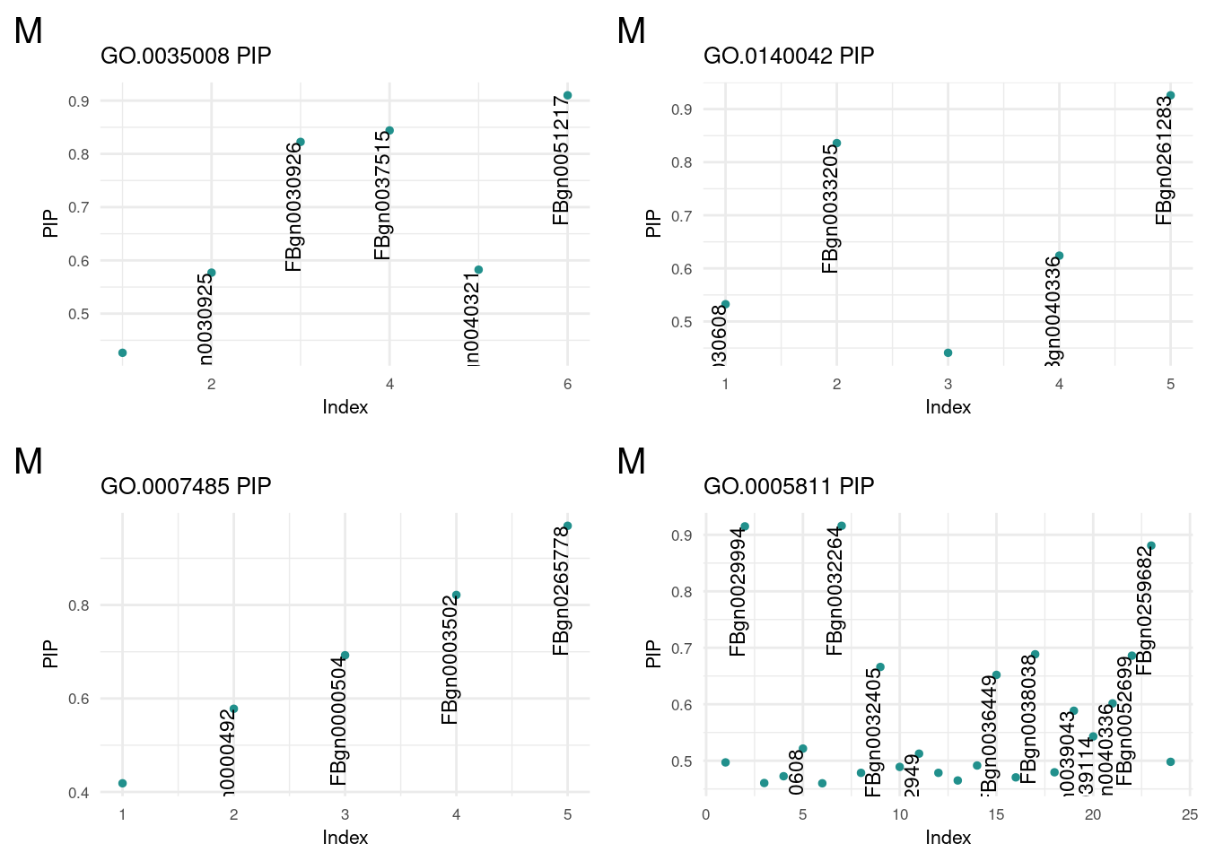
Posterior Inclusion Probability of non-GO portion
plot_grid(nm1, nm2, nm3, nm4, ncol=2)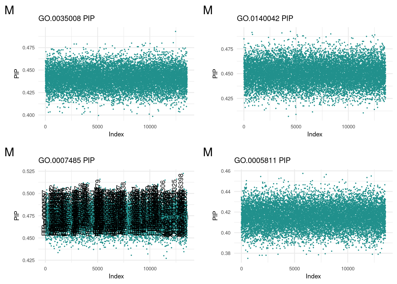
A detailed look at all PIP plots can be found here.
No extreme outlier was found in males.
We then translated the top GO terms into human readable categories to assess our findings. Below are the top ten ordered by correlation:
id: GO:0035008 name: positive regulation of melanization defense response
id: GO:0140042 name: lipid droplet formation
id: GO:0007485 name: imaginal disc-derived male genitalia development
id: GO:0005811 name: lipid droplet
id: GO:0045819 name: positive regulation of glycogen catabolic process
id: GO:0042461 name: photoreceptor cell development
id: GO:0033500 name: carbohydrate homeostasis
id: GO:0016327 name: apicolateral plasma membrane
id: GO:0045186 name: zonula adherens assembly
id: GO:0035003 name: subapical complex
Post-processing
Beyond this, we took the models to determine if certain genes were enriched in the GO terms of interest. From the terms above the cutoff, we pooled the associated genes and totaled gene occurrence.
Females: Out of 323 genes, 37 appeared more than once and 14 appeared twice or more.
Males: Out of 448 genes, 50 appeared more than once and 14 appeared twice or more.
After establishing unique genes, we translated the FlyBase gene codes to human-readable genes.
geneMatchF <- readRDS('snake/goPost/finalDataF.Rds')
geneMatchM <- readRDS('snake/goPost/finalDataM.Rds')

hitF <- geneMatchF[which(count>2),]
hitM <- geneMatchM[which(count>2),]

parm <- dim(hitM)[1] - dim(hitF)[1]

filler <- data.table(matrix(rep(NA, 3*parm), ncol=3))

hitF <- rbind(hitF, filler, use.names=FALSE)

d1 <- cbind(hitF, hitM)

colnames(d1) <- c('Female Gene', 'Count', 'Gene', 'Male Gene', 'Count', 'Gene')

options(knitr.kable.NA = '')

kable(d1, caption = 'Top Female and Male Genes', "simple")| Female Gene | Count | Gene | Male Gene | Count | Gene |
|---|---|---|---|---|---|
| FBgn0025595 | 8 | AkhR | FBgn0261873 | 9 | sdt |
| FBgn0000575 | 7 | emc | FBgn0025595 | 6 | AkhR |
| FBgn0004552 | 4 | Akh | FBgn0067864 | 6 | Patj |
| FBgn0283499 | 4 | InR | FBgn0261854 | 6 | aPKC |
| FBgn0003731 | 4 | Egfr | FBgn0265778 | 5 | PDZ-GEF |
| FBgn0000490 | 4 | dpp | FBgn0036046 | 5 | Ilp2 |
| FBgn0003205 | 4 | Ras85D | FBgn0283499 | 5 | InR |
| FBgn0262738 | 4 | norpA | FBgn0026192 | 5 | par-6 |
| FBgn0010303 | 3 | hep | FBgn0259685 | 4 | crb |
| FBgn0015279 | 3 | Pi3K92E | FBgn0263289 | 4 | scrib |
| FBgn0033799 | 3 | GLaz | FBgn0003391 | 4 | shg |
| FBgn0036449 | 3 | bmm | FBgn0086687 | 4 | Desat1 |
| FBgn0003463 | 3 | sog | FBgn0036449 | 3 | bmm |
| FBgn0003719 | 3 | tld | FBgn0004552 | 3 | Akh |
| FBgn0003205 | 3 | Ras85D | |||
| FBgn0015279 | 3 | Pi3K92E | |||
| FBgn0041191 | 3 | Rheb | |||
| FBgn0002121 | 3 | l(2)gl | |||
| FBgn0011661 | 3 | Moe | |||
| FBgn0000163 | 3 | baz | |||
| FBgn0024248 | 3 | chico |
The following six genes are implicated in both male and female prediction.
Adipokinetic hormone + receptor:
Insulin Receptor pathway:
Others:
sessionInfo()R version 4.1.2 (2021-11-01)
Platform: x86_64-pc-linux-gnu (64-bit)
Running under: Rocky Linux 8.5 (Green Obsidian)
Matrix products: default
BLAS/LAPACK: /opt/ohpc/pub/libs/gnu9/openblas/0.3.7/lib/libopenblasp-r0.3.7.so
locale:
[1] LC_CTYPE=en_US.UTF-8 LC_NUMERIC=C
[3] LC_TIME=en_US.UTF-8 LC_COLLATE=en_US.UTF-8
[5] LC_MONETARY=en_US.UTF-8 LC_MESSAGES=en_US.UTF-8
[7] LC_PAPER=en_US.UTF-8 LC_NAME=C
[9] LC_ADDRESS=C LC_TELEPHONE=C
[11] LC_MEASUREMENT=en_US.UTF-8 LC_IDENTIFICATION=C
attached base packages:
[1] stats graphics grDevices utils datasets methods base
other attached packages:
[1] knitr_1.43 reshape2_1.4.4 melt_1.10.0 ggcorrplot_0.1.4.1
[5] lubridate_1.9.3 forcats_1.0.0 stringr_1.5.0 purrr_1.0.1
[9] readr_2.1.4 tidyr_1.3.0 tibble_3.2.1 tidyverse_2.0.0
[13] scales_1.2.1 viridis_0.6.4 viridisLite_0.4.2 qqman_0.1.9
[17] cowplot_1.1.1 ggplot2_3.4.4 data.table_1.14.8 dplyr_1.1.3
[21] workflowr_1.7.1
loaded via a namespace (and not attached):
[1] Rcpp_1.0.11 getPass_0.2-2 ps_1.7.5 rprojroot_2.0.3
[5] digest_0.6.33 utf8_1.2.3 plyr_1.8.9 R6_2.5.1
[9] evaluate_0.21 highr_0.10 httr_1.4.7 pillar_1.9.0
[13] rlang_1.1.1 rstudioapi_0.15.0 whisker_0.4.1 callr_3.7.3
[17] jquerylib_0.1.4 rmarkdown_2.23 labeling_0.4.3 munsell_0.5.0
[21] compiler_4.1.2 httpuv_1.6.12 xfun_0.39 pkgconfig_2.0.3
[25] htmltools_0.5.5 tidyselect_1.2.0 gridExtra_2.3 fansi_1.0.4
[29] calibrate_1.7.7 tzdb_0.4.0 withr_2.5.0 later_1.3.1
[33] MASS_7.3-60 grid_4.1.2 jsonlite_1.8.7 gtable_0.3.4
[37] lifecycle_1.0.3 git2r_0.32.0 magrittr_2.0.3 cli_3.6.1
[41] stringi_1.7.12 cachem_1.0.8 farver_2.1.1 fs_1.6.3
[45] promises_1.2.0.1 bslib_0.5.0 generics_0.1.3 vctrs_0.6.4
[49] tools_4.1.2 glue_1.6.2 hms_1.1.3 processx_3.8.2
[53] fastmap_1.1.1 yaml_2.3.7 timechange_0.2.0 colorspace_2.1-0
[57] sass_0.4.7