BayesC + Gene Ontology
Last updated: 2023-10-31
Checks: 7 0
Knit directory: dgrp-starve/
This reproducible R Markdown analysis was created with workflowr (version 1.7.1). The Checks tab describes the reproducibility checks that were applied when the results were created. The Past versions tab lists the development history.
Great! Since the R Markdown file has been committed to the Git repository, you know the exact version of the code that produced these results.
Great job! The global environment was empty. Objects defined in the global environment can affect the analysis in your R Markdown file in unknown ways. For reproduciblity it’s best to always run the code in an empty environment.
The command set.seed(20221101) was run prior to running the code in the R Markdown file. Setting a seed ensures that any results that rely on randomness, e.g. subsampling or permutations, are reproducible.
Great job! Recording the operating system, R version, and package versions is critical for reproducibility.
Nice! There were no cached chunks for this analysis, so you can be confident that you successfully produced the results during this run.
Great job! Using relative paths to the files within your workflowr project makes it easier to run your code on other machines.
Great! You are using Git for version control. Tracking code development and connecting the code version to the results is critical for reproducibility.
The results in this page were generated with repository version 6adcbc0. See the Past versions tab to see a history of the changes made to the R Markdown and HTML files.
Note that you need to be careful to ensure that all relevant files for the analysis have been committed to Git prior to generating the results (you can use wflow_publish or wflow_git_commit). workflowr only checks the R Markdown file, but you know if there are other scripts or data files that it depends on. Below is the status of the Git repository when the results were generated:
Ignored files:
    Ignored:    .snakemake/
    Ignored:    code/methodComp/bglr/err-bglr-f.5381.err
    Ignored:    code/methodComp/bglr/err-bglr-m.5382.err
    Ignored:    code/methodComp/m/meth-m.4676.err
    Ignored:    code/methodComp/m/meth-m.4685.err
    Ignored:    code/methodComp/method-f.4751.out
    Ignored:    data/fb/
    Ignored:    data/snake/
    Ignored:    snake/.snakemake/
    Ignored:    snake/ReadMe.md
    Ignored:    snake/Snakefile.yaml
    Ignored:    snake/bayesCheck.R
    Ignored:    snake/bayesTest.Rds
    Ignored:    snake/binner2.R
    Ignored:    snake/code/misc/
    Ignored:    snake/data/
    Ignored:    snake/dgrp.yaml
    Ignored:    snake/h2_synth.R
    Ignored:    snake/labMake.R
    Ignored:    snake/logs/
    Ignored:    snake/slurm/
    Ignored:    snake/snakemake_submitter.sbatch
    Ignored:    snake/zz_lost/
    Ignored:    zz_lost/

Untracked files:
    Untracked:  forester.R
    Untracked:  snake/code/binner.R
    Untracked:  snake/code/combine_GO.R
    Untracked:  snake/code/dataFinGO.R
    Untracked:  snake/code/filterNcombine_GO.R
    Untracked:  snake/code/filter_GO.R
    Untracked:  snake/code/method/bayesHome.R
    Untracked:  snake/code/method/multiplotGO.Rmd

Unstaged changes:
    Modified:   analysis/Method/BayesC.Rmd
    Modified:   analysis/allHist.Rmd
    Modified:   snake/code/method/bayesGO.R
Note that any generated files, e.g. HTML, png, CSS, etc., are not included in this status report because it is ok for generated content to have uncommitted changes.
These are the previous versions of the repository in which changes were made to the R Markdown (analysis/bigGO.Rmd) and HTML (docs/bigGO.html) files. If you’ve configured a remote Git repository (see ?wflow_git_remote), click on the hyperlinks in the table below to view the files as they were in that past version.
| File | Version | Author | Date | Message |
|---|---|---|---|---|
| Rmd | 6adcbc0 | nklimko | 2023-10-31 | wflow_publish(“analysis/bigGO.Rmd”) |
#plotmaker funciton----
ggMake <- function(data, sex, yint, custom.title, custom.Xlab, custom.Ylab){
  plothole <- ggplot(data,aes(y=cor,x=term,color=rgo))+
    geom_point()+scale_color_viridis(begin = 0.1, end=0.9,discrete=TRUE) +
    geom_hline(yintercept = yint) +
    theme_minimal() +
    labs(x=custom.Xlab,y=custom.Ylab, tag=sex, title=custom.title) +
    theme(axis.text.x = element_text(angle = -45, size=10),
          text=element_text(size=10),
          plot.tag = element_text(size=15))
  return(plothole)
}

allMake <- function(data, sex, yint1, yint2, custom.title, custom.Xlab, custom.Ylab){
  plothole <- ggplot(data,aes(y=cor,x=term,color=rgo))+
    geom_point()+scale_color_viridis(begin = 0.1, end=0.9,discrete=TRUE) +
    geom_hline(yintercept = yint1) +
    geom_hline(yintercept = yint2) +
    theme_minimal() +
    labs(x=custom.Xlab,y=custom.Ylab, tag=sex, title=custom.title) +
    theme(axis.text.x = element_text(angle = -45, size=10),
          text=element_text(size=10),
          plot.tag = element_text(size=15))
  return(plothole)
}

rmaxMake <- function(data, sex, custom.title, custom.Xlab, custom.Ylab){
  plothole <- ggplot(data,aes(y=cor,x=term,color=rmax))+
    geom_point()+scale_color_viridis(begin = 0.1, end=0.9,discrete=TRUE) +
    theme_minimal() +
    labs(x=custom.Xlab,y=custom.Ylab, tag=sex, title=custom.title) +
    theme(axis.text.x = element_text(angle = -45, size=10),
          text=element_text(size=10),
          plot.tag = element_text(size=15))
  return(plothole)
}

sortHist <- function(data, sex, yint, custom.title, custom.Xlab, custom.Ylab){
  plothole <- ggplot(data,aes(x=cor))+
    geom_histogram(bins=50) +
    geom_vline(xintercept = yint) +
    theme_minimal() +
    labs(x=custom.Xlab,y=custom.Ylab, tag=sex, title=custom.title) +
    theme(axis.text.x = element_text(angle = -45, size=10),
          text=element_text(size=10),
          plot.tag = element_text(size=15))
  return(plothole)
}
temp <- na.omit(readRDS('snake/data/sr/40_all/go/sexf/allData.Rds'))
facs <- matrix(as.factor(unlist(temp[,1:4])), ncol=4)
cors <- as.numeric(unlist(temp[,5]))
data <- data.table(facs, cors)
colnames(data) <- c('sex', 'rmax', 'rgo', 'term', 'cor')
dataM <- data[data$sex=='m',]
dataF <- data[data$sex=='f',]
yintData1 <- readRDS('snake/data/sr/33_metric/go/sexf/rmax0.8/rgo0/term1/rowData.Rds')
yintData2 <- readRDS('snake/data/sr/33_metric/go/sexm/rmax0.8/rgo0/term1/rowData.Rds')
yF <- as.numeric(yintData1[5])
yM <- as.numeric(yintData2[5])
gg[[1]] <- ggMake(dataF, 'F', yF, 'Effect of R2 Selection on Accuracy by GO Term', 'GO Term', 'Prediction Accuracy')
gg[[2]] <- ggMake(dataM, 'M', yM, 'Effect of R2 Selection on Accuracy by GO Term', 'GO Term', 'Prediction Accuracy')
gg[[3]] <- allMake(data, 'A', yF, yM, 'Effect of R2 Selection on Accuracy by GO Term', 'GO Term', 'Prediction Accuracy')
gg[[4]] <- rmaxMake(data, 'A', 'Effect of Max R2 on Accuracy by GO Term', 'GO Term', 'Prediction Accuracy')
#The data we have here is a few things. The idea behind this work was to analyze the effects of GO terms asa Bayesian prior. By using two separate priors, we aset the first one to efffects of the go terms and the second to the ffects of all non go terms.
#gg[[4]] <- rmaxMake(data, 'A', 'Effect of Max R2 on Accuracy by GO Term', 'GO Term', 'Prediction Accuracy')
#colnames(hold) <- c("method", "cor")
#hold$method <- factor(hold$method, levels=unique(hold$method))
#for when the first works for sure, copy paste to compare and see if it mattered at all
#ggplot(data,aes(y=cor,x=term,color=rgo))+For both females and males, a random selection of Gene Ontology(GO) terms were used to subset transcriptomic data from fruit flies.
The model used to calculate prediction accuracy uses two BayesC priors using the GO-associated genes as a discriminator.
By changing the proportion of variance explained by the GO-associated prior(R2_GO), we sought to find gene clusters that would improve overall prediction accuracy.
The following data points are all point means of 25 replicates at 5-fold cross-validation.
plot_grid(gg[[1]],gg[[2]], ncol=1)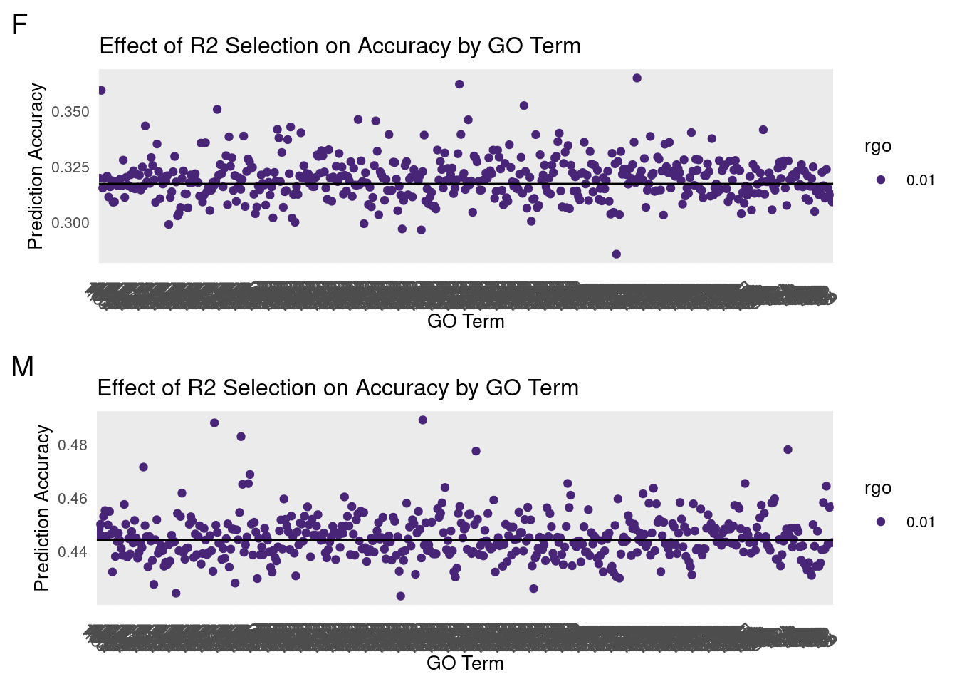
#Data prep 2

gg[[5]] <- sortHist(dataF, 'F', yF, 'Prediction Accuracy Histogram', 'Prediction Accuracy', 'Count')
gg[[6]] <- sortHist(dataM, 'M', yM, 'Prediction Accuracy Histogram', 'Prediction Accuracy', 'Count')


#plot(dataM[order(cor),cor])
#abline(h=c(0.32, 0.35, 0.465, 0.44))

query <- readRDS("snake/data/go/query.Rds")

subF <- dataF[cor>0.35,4:5]
trueF <- query[as.numeric(subF[,term])]
subF <- data.table(trueF, subF[,cor])
colnames(subF) <- c('term','cor')
subF <- subF[order(-cor),]


subM <- dataM[cor>0.47,4:5]
trueM <- query[as.numeric(subM[,term])]
subM <- data.table(trueM, subM[,cor])
colnames(subM) <- c('term','cor')
subM <- subM[order(-cor),]
Histograms of Both
plot_grid(gg[[5]],gg[[6]], ncol=1)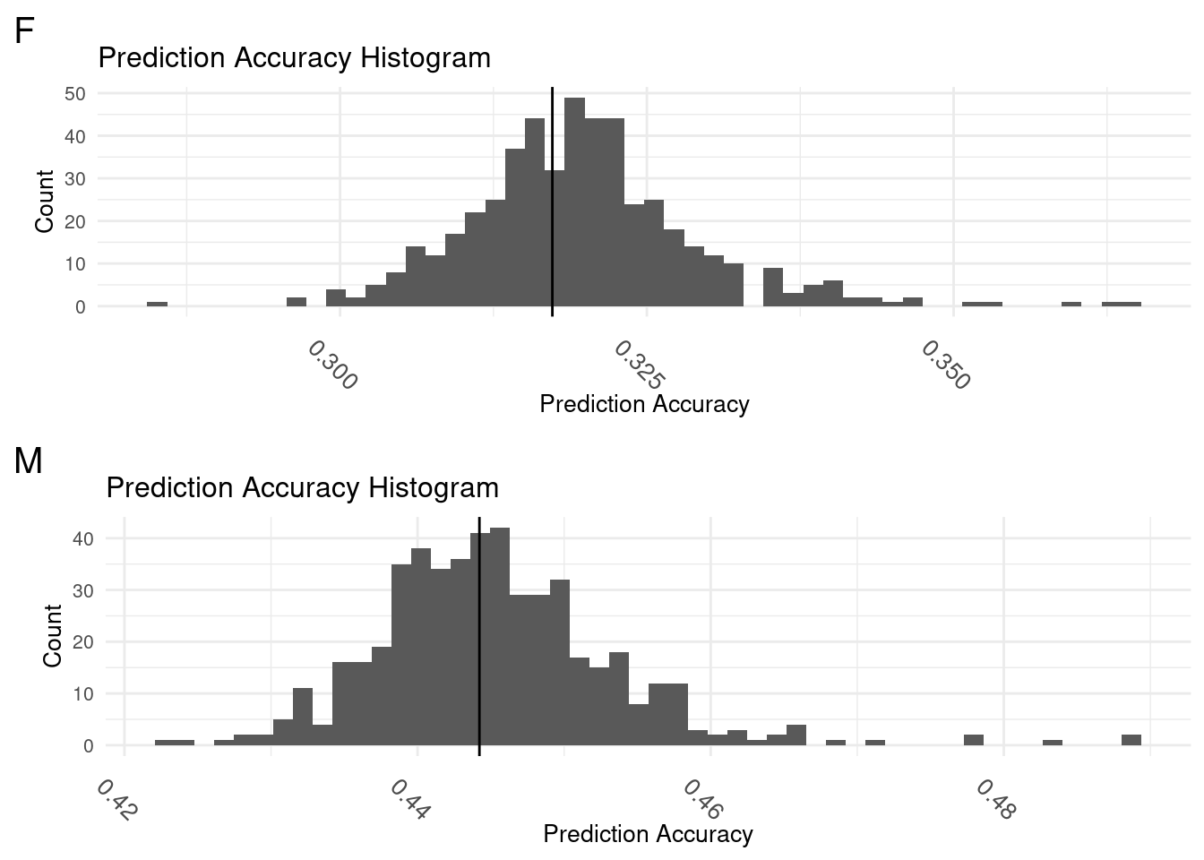
Cutoff of 0.3 for both
plot(dataF[order(cor),cor])
abline(h=c(0.32, 0.35))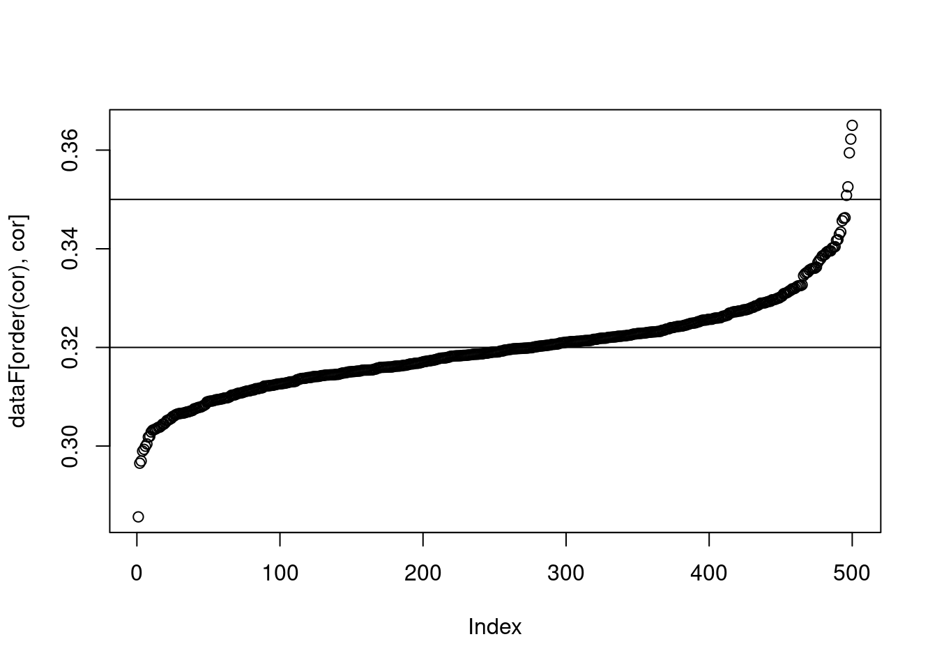
plot(dataM[order(cor),cor])
abline(h=c(0.44, 0.47))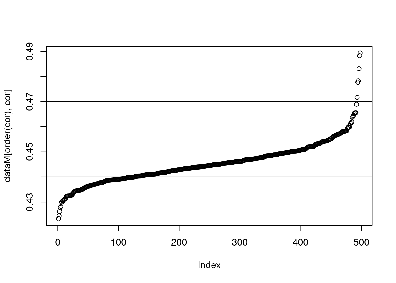
The vertical lines on each graph indicate the prediction accuracy of the base model. A normal distribution of prediction accuracy values are centered on the base model for both.
Filtering for an improvement of 0.03 or higher yields the following GO terms of significance:
- In females:
print(subF) term cor
1: GO.00000011253 0.3650187
2: GO.000000158 0.3622343
3: GO.000000123 0.3594467
4: GO.000000163 0.3525587
5: GO.0000001350 0.3508321- In males:
print(subM) term cor
1: GO.0000001806 0.4893254
2: GO.0000001349 0.4882313
3: GO.0000001389 0.4830880
4: GO.0000001121 0.4782296
5: GO.000000159 0.4776605
6: GO.0000001235 0.4716803
sessionInfo()R version 4.1.2 (2021-11-01)
Platform: x86_64-pc-linux-gnu (64-bit)
Running under: Rocky Linux 8.5 (Green Obsidian)
Matrix products: default
BLAS/LAPACK: /opt/ohpc/pub/libs/gnu9/openblas/0.3.7/lib/libopenblasp-r0.3.7.so
locale:
[1] LC_CTYPE=en_US.UTF-8 LC_NUMERIC=C
[3] LC_TIME=en_US.UTF-8 LC_COLLATE=en_US.UTF-8
[5] LC_MONETARY=en_US.UTF-8 LC_MESSAGES=en_US.UTF-8
[7] LC_PAPER=en_US.UTF-8 LC_NAME=C
[9] LC_ADDRESS=C LC_TELEPHONE=C
[11] LC_MEASUREMENT=en_US.UTF-8 LC_IDENTIFICATION=C
attached base packages:
[1] stats graphics grDevices utils datasets methods base
other attached packages:
[1] reshape2_1.4.4 melt_1.10.0 ggcorrplot_0.1.4.1 lubridate_1.9.2
[5] forcats_1.0.0 stringr_1.5.0 purrr_1.0.1 readr_2.1.4
[9] tidyr_1.3.0 tibble_3.2.1 tidyverse_2.0.0 scales_1.2.1
[13] viridis_0.6.4 viridisLite_0.4.2 qqman_0.1.9 cowplot_1.1.1
[17] ggplot2_3.4.3 data.table_1.14.8 dplyr_1.1.3 workflowr_1.7.1
loaded via a namespace (and not attached):
[1] Rcpp_1.0.11 getPass_0.2-2 ps_1.7.5 rprojroot_2.0.3
[5] digest_0.6.33 utf8_1.2.3 plyr_1.8.8 R6_2.5.1
[9] evaluate_0.21 highr_0.10 httr_1.4.7 pillar_1.9.0
[13] rlang_1.1.1 rstudioapi_0.15.0 whisker_0.4.1 callr_3.7.3
[17] jquerylib_0.1.4 rmarkdown_2.23 labeling_0.4.3 munsell_0.5.0
[21] compiler_4.1.2 httpuv_1.6.11 xfun_0.39 pkgconfig_2.0.3
[25] htmltools_0.5.5 tidyselect_1.2.0 gridExtra_2.3 fansi_1.0.4
[29] calibrate_1.7.7 tzdb_0.4.0 withr_2.5.0 later_1.3.1
[33] MASS_7.3-60 grid_4.1.2 jsonlite_1.8.7 gtable_0.3.4
[37] lifecycle_1.0.3 git2r_0.32.0 magrittr_2.0.3 cli_3.6.1
[41] stringi_1.7.12 cachem_1.0.8 farver_2.1.1 fs_1.6.3
[45] promises_1.2.0.1 bslib_0.5.0 generics_0.1.3 vctrs_0.6.3
[49] tools_4.1.2 glue_1.6.2 hms_1.1.3 processx_3.8.2
[53] fastmap_1.1.1 yaml_2.3.7 timechange_0.2.0 colorspace_2.1-0
[57] knitr_1.43 sass_0.4.7